

![]()
![]()
![]()
Physical oceanography is an experimental science and requires observation and exact measurement to achieve its aims. It can draw on the experience of the related science fields of physics and chemistry and make use of existing achievements in the areas of technology and engineering, but the oceanic environment places unique demands on instrumentation that are not easily met by standard laboratory equipment. As a consequence, the development and manufacturing of oceanographic instrumentation developed into a specialised activity. Manufacturers of oceanographic equipment serve a small market but aim at selling their products world-wide.
This lecture gives an overview of the range of instrumentation used at sea and the principles involved. It aims at covering standard classical instruments as well as modern developments. The following table summarises its content.
| research need | available equipment / instrumentation |
|---|---|
| provision of observing platform |
|
| measurement of hydrographic properties (temperature, salinity, oxygen, nutrients, tracers) |
|
| measurement of dynamic properties (currents, waves, sea level, mixing processes) |
|
All measurements at sea require a reasonably stable platform to carry the necessary instrumentation. The platform can be at the sea surface, at the sea floor, in the ocean interior or in space. The choice of platform depends on its capabilities to collect the required information in space and time.
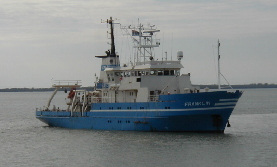 Figure 13.1
Like any other ocean going ship, research vessels have to meet the requirement to be seaworthy and capable of riding out bad weather. The weather conditions in the investigation area thus define the minimum size for the vessel. Additional requirements, such as the handling of heavy equipment at sea or the need for a large scientific party during an interdisciplinary study, can increase the minimum size. Typical ocean going research vessels are 50 - 80 m long, have a total displacement of 1000 - 2000 tonnes and provide accommodation for 10 - 20 scientists (Figure 13.1).
The shape of a research vessel is determined by the need for a reasonably large working deck, several powerful winches for lowering and retrieving instrumentation and at least one "A-frame", a structure which allows a wire to go from the ship's winch over the side of the ship or over the stern and vertically into the water (Figure 13.2).
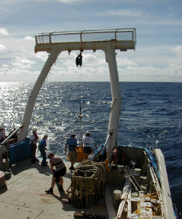 Figure 13.2
The requirement to be at sea for extensive periods of time, remain stationary while equipment is handled over the side and move at very slow speed when equipment is towed behind the vessel place additional demands on research vessel design. To increase endurance (the number of days a ship can remain at sea before running out ouf fuel), research vessels have only a moderate operating speed of 10 - 12 knots (18 - 28 km/hr). This compares with operating speeds of 15 - 20 knots for merchant ships. Most research vessels have an endurance of 20 - 25 days, which gives them a range of 6000 - 8000 nautical miles (11,000 - 14,800 km), sufficient to operate at the high seas within a few days of reach of land. Only the major oceanographic institutions of the world operate research vessels with global research capability.
All modern ships are powered by Diesel engines. Such engines are best operated at nearly constant speed. Merchant ships do not have to vary their speed much during their voyage; their propeller is diven directly from the engine. Various arrangements are used to allow research vessels to operate at very slow speeds. In diesel-electric systems the Diesel engine powers an electic motor which in turn drives the propeller shaft. Electric motors work efficiently at any speed, allowing the ship very accurate speed control. In another arrangement the Diesel engine drives a "variable pitch propeller". In such a propeller the pitch of the blades (the blade angle) can be controlled to give very low or zero propeller thrust even at full propeller rotation.
Lowering equipment over the side of a vessel requires more than zero thrust. Without active position control the ship will drift with the wind and across the instrument wire. To keep the wire vertical and free from the ship's hull the ship has to counteract the effects of wind and current. This is usually achieved through a pair of additional thrusters, one at the bow and one at the stern, which can push the ship sideways. The bow thruster is either a propeller set into a horizontal tunnel through the ship's hull or a propeller on a shaft that can be oriented in any direction and retracted when the ship is under way. The stern thruster is either a similar tunnel or a propeller built into the ship's rudder (an "active rudder"). The two thrusters together allow very accurate control over the ship's behaviour in wind, waves and current and enable it to turn itself around on the spot if neccessary.
 Figure 13.3
The minimum laboratory requirements consist of a wet laboratory for the handling of water samples, a computer laboratory for data processing, an electronics laboratory for the preparation of instruments and a chemical laboratory for water sample analysis. Larger research vessels designed for multidisciplinary research have additional biological, geophysical and geological laboratories. Figure 13.3 shows a typical deck arrangement on a medium sized research vessel.
Research vessels are expensive to operate (US$15,000 - US$25,000 per day at sea). For many decades they were the only available type of platform for data collection on the high seas. The advent of deep-sea moorings, satellites and autonomous drifters has reduced their importance, but research vessels still are an essential tool in oceanographic research. They are now used principally for large scale near-synoptic surveys of oceanic property fields and for targeted process studies (such as mixing across fronts, determination of the heat budget of small ocean regions etc).
Moorings are appropriate platforms wherever measurements are required at one location over an extended time period. Their design depends on the water depth and on the type of instrumentation for which the mooring is deployed, but the basic elements of an oceanographic mooring are an anchor, a mooring line (wire or rope) and one or more buoyancy elements which hold the mooring upright and preferably as close to vertical as possible.
 Figure 13.4
Subsurface moorings are used in deep water in situations where information about the surface layer is not essential to the experiment. The main buoyancy at the top of the mooring line is placed some 20 - 50 m below the ocean surface. This has the advantage that the mooring is not exposed to the action of surface waves and is not at risk of being damaged by ship traffic or being vandalised or stolen. Figure 13.4 shows a typical deep-sea mooring. The main buoyancy is at the top of the mooring line. To protect the mooring against fish bites, wire is used for the upper 1000 m or so of the mooring line, while rope is used below.
To keep the mooring close to the vertical it should have minimum drag, which can only be achieved by keeping the wire diameter small. This requires a small wire load from the instruments. Additional buoyancy is therefore distributed along the wire to compensate for the weight of the instrumentation. The buoyancy is arranged so that all sections of thew mooring are buoyant, enabling recovery of a damaged mooring which lost its upper part.
At the bottom of a deep sea mooring just above the anchor is a remotely controllable release. It can be activated through a coded acoustic signal from the ship when it is time to recover the mooring. Triggering the release brings the mooring to the surface. The anchor, usually a concrete block or a clump of disused railway wheels, is left at the ocean floor.
 Figure 13.5
An experiment which includes the surface layer or the collection of meteorological data requires a surface mooring. The main buoyancy for such a mooring takes the shape of a substantial buoy that floats at the surface and can carry meteorological instrumentation (Figure 13.5). In the deep ocean surface moorings are mostly "taut moorings". They use only rope for the mooring line and make it a few per cent shorter than the water depth. This stretches the rope and keeps it under tension to keep the mooring close to vertical. The "inverse catenary" mooring is also used; this is an arrangement where a buoyant section of mooring line is included between two non-buoyant sections causing the profile of the line to form an S-shape. In this configuration the length of the mooring line is not critical and is about 25% greater than the water depth.
 Figure 13.6
Moorings on the continental shelf, where the water depth does not exceed 200 m, do not require acoustic releases if a U-type mooring is used. A U-type mooring consists of a surface or subsurface mooring to carry the instrumentation, a ground line of roughly twice the water depth and a second mooring with a small marker buoy (Figure 13.6). When the time comes to bring the mooring in, the marker buoy is recovered first, followed by the two anchors and finally the mooring itself. U-type moorings are usually "slack moorings"; the mooring line is longer than the water depth, and the mooring swings with the current.
The advent of satellite technology opened the possibility of measuring some property fields and dynamic quantities from space. The advantage of this method is the nearly synoptic coverage of entire oceans and ease of access to remote ocean regions. Satellites have therefore become an indispensable tool for climate research. The major restriction of the method is that satellites can only see the surface of the ocean and therefore give only limited information about the ocean interior.
Most satellites are named for the sensors they carry. Strictly speaking, the satellite and its sensors are two separate things; the satellite is a platform, the sensors are instruments. An overview of the available satellite sensors is therefore given in the discussion of instruments below.
As platforms, satellites fall into three groups. Most satellites follow inclined orbits: Their elliptical orbits are inclined against the equator. The degree of inclination determines how far away from the equator the satellite can see the Earth. Typical inclinations are close to 60º, so the satellite covers the region from 60ºN to 60ºS. It covers this region frequently, completing one orbit around the Earth in about 50 minutes.
Some satellites have an inclination of nearly or exactly 90º and can therefore see both poles; they fly on polar orbits. A typical height of satellites on polar and on inclined orbits is 800 km.
The third and last group are the geostationary satellites. They orbit the Earth at the same speed with which the Earth rotates around its axis and are therefore stationary with respect to the Earth. This situation is only possible if the satellite is over the equator and orbits at a height of 35,800 km, much higher than all other satellites. Geostationary satellites therefore cannot see the poles.
The selection of a satellite as a platform logically includes the selection of a sensor and a suitable orbit. An ice sensor to monitor the polar ice caps does not achieve much on a geostationary satellite; a cloud imager for weather forecasting is not placed in a polar orbit.
Submersibles are not a frequently used platform in physical oceanography, but this is likely to change over the coming years. Three basic types can be distinguished, manned submersibles, remotely controlled submersibles and autonomous submersibles.
Manned submersibles are used in marine geology for the exploration of the sea floor and occasionally in marine biology to study sea floor ecosystems. They are not a tool for physical oceanography.
Remotely controlled submersibles are commonly used in the offshore oil and gas industry and for retrieving flight recorders from aircraft that fell into the ocean. In science they find similar uses to manned submersibles but are again not a tool for physical oceanography.
Autonomous submersibles are self-propelled vehicles that can be programmed to follow a predetermined diving path. Such vehicles have great potential for physical oceanography. Some major oceanographic research institutions are developing vehicles to carry instrumentation such as a CTD and survey an ocean area by regularly diving and surfacing along a track from one side of an ocean region to the other and transmitting the collected data via satellite when at the surface. Some time will pass, however, before these vehicles will come into regular use. Eventually, autonomous submersibles will greatly reduce the need for research vessels for ocean monitoring.
Towed vehicles are used from research vessels to study oceanic processes which require high spatial resolution such as mixing in fronts and processes in the highly variable upper ocean. Most systems consist of a hydrodynamically shaped underwater body, an electro-mechanical (often multi-conductor) towing cable and a winch. The underwater body is fitted with a pair of wing shaped fins which control its flight through the water. In addition to the sensor package (usually a CTD, sometimes additional sensors for chemical measurements) it carries sensors for pressure, pitch and roll to monitor its behaviour and control its flight. The data are sent to the ship's computer system via the cable. The same cable is used to send commands to the underwater body to alter its wing angle.
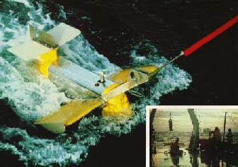 Figure 13.7
Figure 13.7 shows a towed vehicle during deployment. A typical flight path for this vehicle covers a depth range of about 250 - 500 m, which can be chosen to be anywhere between the surface and 800 m depth. The vehicle is towed at about 6 - 10 knots (10 - 18 km/h) and traverses the 250 m depth range about once every 5 minutes. When fitted with a CTD this results in a vertical section of temperature and salinity with a horizontal resolution of about 1 km.
An alternative towed system does not employ an underwater body to carry the sensor package but has sensors (for example thermistors) built into the towed cable at fixed intervals. Because the distance between the sensors is fixed and the sensors remain at the same depth during the tow, these "thermistor chains" do not offer the same vertical data resolution as undulating towed systems and are only rarely used now.
The main characteristic of floats and drifters is that they move freely with the ocean current, so their position at any given time can only be controlled in a very limited way. Until a decade ago these platforms were mainly used in remote regions such as the Southern Ocean and in the central parts of the large ocean basins that are rarely reached by research vessels and where it is difficult and expensive to deploy a mooring. They have now become the backbone of a new observing system that covers the entire ocean.
Strictly speaking, a float is a generic term for anything that does not sink to the ocean floor. A drifter, on the other hand, is a platform designed to move with the ocean current. To achieve this it has to incorporate a floatation device or float, but it is usually more than that. But oceanographers use the terms very loosely and do not make a clear distinction between "floats" and "drifters".
 Figure 13.8
Two basic types can be distinguished. Surface drifters have a float at the surface and can therefore transmit data via satellite. If they are designed to collect information about the ocean surface they carry meteorological instruments on top of the float and a temperature and occasionally a salinity sensor underneath the float. To prevent them from being blown out of the area of interest by strong winds they are fitted with a "sea anchor" at some depth (Figure 13.8). If they are designed to give information on subsurface ocean properties, additional sensors are placed between the surface float and the sea anchor. The depth range of surface drifters is usually limited to less than 100 m.
Floats used for subsurface drifters are designed to be neutrally buoyant at a selected depth. These drifters have been used to follow ocean currents at various depths, from a few hundred metres to below 1000 m depth. The first such floats transmitted their data acoustically through the ocean to coastal receiving stations. Because sound travels well at the depth of the sound velocity minimum (the SOFAR channel), these SOFAR floats can only be used at about 1000 m depth.
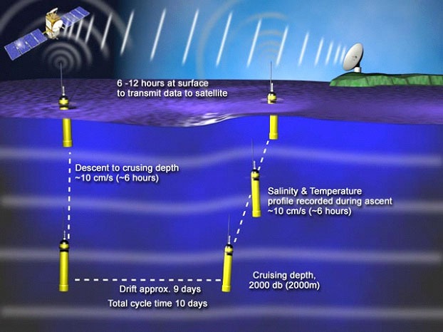 Figure 13.8a
Modern subsurface floats remain at depth for aperiod of time, come to the surface briefly to transmit their data to a satellite and return to their allocated depth. These floats can therefore be programmed for any depth and can also obtain temperature and salinity (CTD) data during their ascent. The most comprehensive array of such floats, known as Argo, began in the year 2000. Argo floats measure the temperature and salinity of the upper 2000 m of the ocean (Figure 13.8a). This will allow continuous monitoring of the climate state of the ocean, with all data being relayed and made publicly available within hours after collection. When the Argo programme is fully operational it will have 3,000 floats in the world ocean at any one time.
This section gives an overview of sensors and instrument packages for the measurement of temperature, salinity, oxygen, nutrients and tracers.
The earliest temperature measurements at some depth below the surface where made by bringing a water sample up to the deck of a ship in an insulated bucket and measuring the sample temperature with a mercury thermometer. Although these measurements were not accurate, they gave the first evidence that below the top 1000 m the ocean is cold even in the tropics. They also showed that highly accurate measurements are required to resolve the small temperature differences between different ocean regions at those depths.
The first instrument that (through the use of multiple sampling and averaging) achieved the required accuracy of 0.001 ºC was the reversing thermometer. It consists of a mercury filled glas pipe with a 360º coil. The pipe is restricted to capillary width in the coil, where it has a capillary appendix (Figure 13.9). The instrument is lowered to the desired depth. Mercury from a reservoir at the bottom rises in proportion to the outside temperature. When the desired depth is reached the thermometer is turned upside down (reversed), but the flow of mercury is now interrupted at the capillary appendix, and only the mercury that was above the break point is collected in the lower part of the glass pipe. This part carries a calibrated gradation that allows the temperature to be read when the thermometer is returned to the surface.
To eliminate the effect of pressure, which compresses the pipe and causes more mercury to rise above the break point during the lowering of the instrument, the thermometer is enclosed in a pressure resistent glass housing. If such a "protected reversing thermometer" is used in conjunction with an "unprotected reversing thermometer" (a thermometer exposed to the effect of pressure), the difference between the two temperature readings can be used to determine the pressure and thus the depth at which the readings were taken. The reversing thermometer is thus also an instrument to measure depth.
Reversing thermometers require a research vessel as platform and are used in conjunction with Nansen or Niskin bottles or on multi-sample devices.
The measurement of salinity and oxygen, nutrients and tracer concentrations requires the collection of water samples from various depths. This essential task is achieved through the use of "water bottles". The first water bottle was developed by Fritjof Nansen and is thus known as the Nansen bottle. It consists of a metal cylinder with two rotating closing mechanisms at both ends. The bottle is attached to a wire (Figure 13.10). When the bottle is lowered to the desired depth it is open at both ends, so the water flows through it freely. At the depth where the water sample is to be taken the upper end of the bottle disconnects from the wire and the bottle is turned upside down. This closes the end valves and traps the sample, which can then be brought to the surface.
 Figure 13.10
In an "oceanographic cast" several bottles are attached at intervals on a thin wire and lowered into the sea. When the bottles have reached the desired depth, a metal weight ("messenger") is dropped down the wire to trigger the turning mechanism of the uppermost bottle. The same mechanism releases a new messenger from the bottle; that messenger now travels down the wire to release the second bottle, and so on until the last bottle is reached.
 Figure 13.11
The Nansen bottle has now widely been displaced by the Niskin bottle (Figure 13.11). Based on Nansen's idea, it incorporates two major modifications. Its cylinder is made from plastic, which eliminates chemical reaction between the bottle and the sample that may interfere with the measurement of tracers. Its closing mechanism no longer requires a turning over of the bottle; the top and bottom valves are held open by strings and closed by an elastic band. Because the Niskin bottle is fixed on the wire at two points instead of one (as is the case with the Nansen bottle) it makes it easier to increase its sample volume. Niskin bottles of different sizes are used for sample collection for various tracers.
Nansen and Niskin bottles are used on conjunction with reversing thermometers. On the Nansen bottle the thermometers are mounted in a fixed frame, the reversal being achieved by the turning over of the bottle. On Niskin bottles thermometers are mounted on a rotating frame.
 Figure 13.12
Today's standard instrument for measuring temperature, salinity and often also oxygen content is the CTD, which stands for conductivity, temperature, depth (Figure 13.12). It employs the principle of electrical measurement. A platinum thermometer changes its electrical resistance with temperature. If it is incorporated in an electrical oscillator, a change in its resistance produces a change of the oscillator frequency, which can be measured. The conductivity of seawater can be measured in a similar way as a frequency change of a second oscillator, and a pressure change produces a frequency change in a third oscillator. The combined signal is sent up through the single conductor cable on which the CTD is lowered. This produces a continuous reading of temperature and conductivity as functions of depth at a rate of up to 30 samples per second, a vast improvement over the 12 data points produced by the 12 Nansen or Niskin bottles that could be used on a single cast.
Electrical circuits allow measurements in quick succession but suffer from "instrumental drift", which means that their calibration changes with time. CTD systems therefore have to be calibrated by comparing their readings regularly against more stable instruments. They are therefore always used in conjunction with reversing thermometers and a multi-sample device.
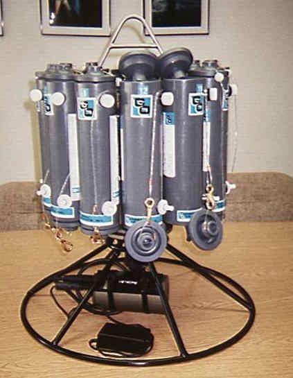 Figure 13.13
Multiple water sample devices allow the use of Niskin bottles on electrically conducting wire. Different manufacturers have different names for their products, such as rosette or carousel. In all products the Niskin bottles are arranged on a circular frame (Figure 13.13), with a CTD usually mounted underneath or in the centre.
The advantage of multi-sample devices over the use of a hydrographic wire with messengers is that the water bottles can be closed by remote control. This means that the sample depths do not have to be set before the bottles are lowered. As the device is lowered and data are received fom the CTD, the operator can look for layers of particular interest and take water samples at the most interesting depth levels.
The introduction of the CTD opened the possibility of taking continuous readings of temperature and salinity at the surface. Water from the cooling water intake of the ship's engines is pumped through a tank in which a temperature and a conductivity sensor are installed. Such a system is called a thermosalinograph.
Most oceanographic measurements from space or aircraft are based on the use of radiometers, instruments that measure the electro-magnetic energy radiating from a surface. This radiation occurs over a wide range of wavelengths, including the emission of light in the visible range, of heat in the infrared range, and at shorter wavelengths such as Radar and X-rays. Most oceanographic radiometers operate in several wavelength bands. A detailed discussion of all applications goes beyond the scope of these lecture notes; so only the most basic systems are mentioned here.
Radiometers that operate in the infrared are used to measure sea surface temperature. Their resolution has steadily increased over the years; the AVHRR (Advanced Very High Resolution Radiometer) has a resolution that comes close to 0.2º C.
Multi-spectral radiometers measure in several wavelength bands. By comparing the radiation signal received at different wavelengths it is possible to measure ice coverage and ice age, chlorophyll content, sediment load, particulate matter and other quantities of interest to marine biology.
Measurements at radar wavelengths are made by an instrument known as SAR (Synthetic Aperture Radar). It can be used to detect surface expressions of internal waves, the effect of rainfall on surface waves, the effect of bottom topography on currents and waves, and a range of other phenomena. Many of these phenomena belong into the category "dynamic properties" discussed below.
All instruments discussed so far produce information about oceanic property fields irrespective of the dynamic state of the ocean. The remainder of this lecture summarises instrumentation designed to measure movement in the ocean.
An elementary way of observing oceanic movement is the use of drifters. As mentioned above, drifters are platforms designed to carry instruments. But all measurements obtained from drifters are of little use unless they can be related to positions in space. A geolocation (GPS) device which transmits the drifter location to a satellite link is therefore an essential instrument on any drifter, and this turns the drifter into an instrument for the measurement of ocean currents. Whether it does that job well or not depends on its design, and in particular the size and shape of its sea anchor.
 Figure 13.14
Ocean currents can be measured in two ways. An instrument can record the speed and direction of the current, or it can record the east-west and north-south components of the current (Figure 13.14). Both methods require directional information. All current meters therefore incorporate a magnetic compass to determine the orientation of the instrument with respect to magnetic north. Four classes of current meters can be distinguished, based on the method used for measuring current magnitude.
Mechanical current meters use a propeller-type device, a Savonius rotor or a paddle-wheel rotor (Figure 13.15) to measure the current speed, and a vane to determine current direction. Propeller sensors often measures speed correctly only if they point into the current and have to be oriented to face the current all the time. Such instruments are therefore fitted with a large vane, which turns the entire instrument and with it the propeller into the current.
 Figure 13.15
Propellers can be designed to have a cosine response with the angle of incidence of the flow. Two such propellers arranged at 90º will resolve current vectors and do not require an orienting vane.
The advantage of the Savonius rotor is that its rotation rate is independent of the direction of exposure to the current. A Savonius rotor current meter therefore does not have to face the current in any particular way, and its vane can rotate independently and be quite small, just large enough to follow the current direction reliably.
With the exception of the current meter that uses two propellers with cosine response set at 90º to each other, mechanical current meters measure current speed by counting propeller or rotor revolutions per unit time and current direction by determining the vane orientation at fixed intervals. In other words, these current meters combine a time integral or mean speed over a set time interval (the number of revolutions between recordings) with an instanteneous reading of current direction (the vane orientation at the time of recording). This gives only a reliable recording of the ocean current if the current changes slowly in time. Such mechanical current meters are therefore not suitable for current measurement in the oceanic surface layer where most of the oceanic movement is due to waves.
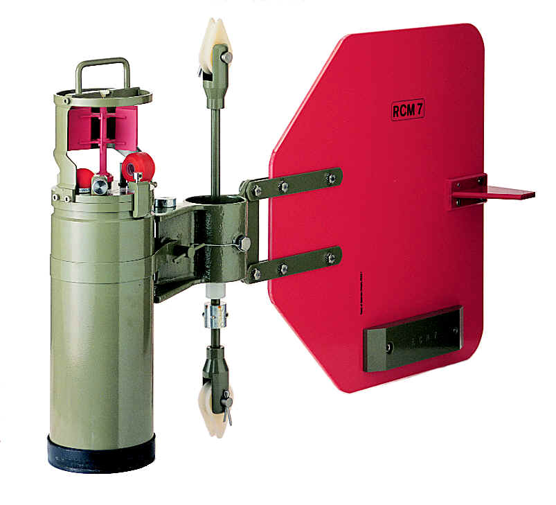 Figure 13.16
The Savonius rotor is particularly problematic in this regard. Suppose that the current meter is in a situation where the only water movement is from waves. The current then alternates back and forth, but the mean current is zero. A Savonius rotor will pick up the wave current irrespective of its direction, and the rotation count will give the impression of a strong mean current. The paddle-wheel rotor is designed to rectify this; the paddle wheel rotates back and forth with the wave current, so that its count represents the true mean current (Figure 13.16).
Mechanical current meters are robust, reliable and comparatively low in cost. They are therefore widely used where conditions are suitable, for example at depths out of reach of surface waves.
Electromagnetic current meters exploit the fact that an electrical conductor moving through a magnetic field induces an electrical current. Sea water is a very good conductor (see Lecture 3), and if it is moved between two electrodes the induced electrical current is proportional to the ocean current velocity between the electrodes. An electromagnetic current meter has a coil to produce a magnetic field and two sets of electrodes, set at right angle to each other, and determines the rate at which the water passes between both sets. By combining the two components the instrument determines speed and direction of the ocean current.
Acoustic current meters are based on the principle that sound is a compression wave that travels with the medium. Assume an arrangement with a sound transmitter between two receivers in an ocean current. Let receiver A be located upstream from the transmitter, and let receiver B located downstream. If a burst of sound is generated at the transmitter it will arrive at receiver B earlier than at receiver A, having been carried by the ocean current.
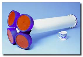 Figure 13.17
A typical acoustic current meter will have two orthogonal sound paths of approximately 100 mm length with a receiver/transmitter at each end. A high frequency sond pulse is transmitted simultaneously from each transducer and the difference in arrival time for the sound travelling in opposite directions gives the water velocity along the path.
Electromagnetic and acoustic current meters have no moving parts and can therefore take measurements at a very high sampling rate (up to tens of readings per second). This makes them useful not only for the measurement of ocean currents but also for wave current and turbulence measurements.
Acoustic doppler current profilers (ADCPs) operate on the same principle as acoustic current meters but have transmitter and receiver in one unit and use reflections of the sound wave from drifting particles for the measurement. Seawater always contains a multitude of small suspended particles and other solid matter that may not all be visible to the naked eye but reflects sound. If sound is transmitted in four inclined beams at right angle to each other, the Doppler frequency shift of the reflected sound gives the reflecting particle velocity along the beam. With at least 3 beams inclined to the vertical the 3 components of flow velocity can be determined. Different arrival times indicate sound reflected at different distances from the transducers, so an ADCP provides information on current speed and direction not just at one point in the ocean but for a certain depth range; in other words, an ADCP produces a current profile over depth.
Different ADCP designs serve different purposes (Figure 13.17). Deep ocean ADCPs have a vertical resolution of typically 8 metres (they produce one current measurement for every 8 metres of depth increase) and a typical range of up to 400 m. ADCPs designed for measurements in shallow water have a resolution of typically 0.5 m and a range of up to 30 m. ADCPs can be placed in moorings, installed in ships for underway measurements, or lowered with a CTD and multi-sample device to give a current profile over a large depth range.
The parameters of interest in the measurement of surface waves are wave height, wave period and wave direction. At locations near the shore wave height and wave period can be measured by using the principle of the stilling well described for tide gauges below, with an opening wide enough to let pass surface waves unhindered. Wave measurements on the shelf but at some distance from the shore can be obtained from a pressure gauge (see under tide gauges as well).
An instrument suitable for all locations including the open ocean is the wave rider, a small surface buoy on a mooring which follows the wave motion. A vertical accelerometer built into the wave rider measures the buoy's acceleration generated by the waves. The data are either stored internally for later retrieval or transmitted to shore. Wave riders provide information on wave height and wave period. If they are fitted with a set of 3 orthogonal accelerometers they also record wave direction.
 Figure 13.18
Tides are waves of long wavelength and known period, so the major properties of interest for measurement are wave height, or tidal range, and wave induced current. The latter is measured with current meters; any type is suitable. Two types of tide gauges are used to measure the tidal range. The stilling-well gauge consists of a cylinder with an connection to the sea at the bottom. This connection acts as a low pass filter: It is so restricted that the backward and forward motion of the water associated with wind waves and other waves of short period cannot pass through; only the slow change of water level associated with the tide can enter the well. This change of water level is picked up by a float and recorded (Figure 13.18).
Stilling-well gauges allow the direct reading of the water level at any time but require a somewhat laborious installation and are impracticable away from the shore. In offshore and remote locations it is often easier to use a pressure gauge. Such an instrument is placed on the sea floor and measures the pressure of the water column above it, which is proportional to the height of water above it. The data are recorded internally and not accessible until the gauge is recovered.
Tide gauges are increasingly used to monitor possible long term changes in sea level linked with climate variability and climate change. The expected rate of sea level change is only a few millimetres per year at most, so very high accuracy is required to verify such changes. Most tide gauges are not suitable for such a task, for a number of reasons. For example, a long term trend in observed sea level can also be produced by a rise or fall of the land on which the tide gauge is built. (This is known as benchmark drift.) The wire in a stilling-well gauge that connects the float with the recording unit stretches and shrinks as the air temperature rises and falls. Such effects are insignificant when the gauge is used to verify the depth of water for shipping purposes but not when it comes to assessing trends of millimetres per year. A new generation of tide gauges is being installed world wide which gives water level recordings to absolute accuracies of a few millimetres with long term benchmark stability. In these instruments the float and wire arrangement of the stilling-well gauge is replaced by a laser distance measurement, and the data are transmitted via satellite to a world sea level centre which monitors the performance of every gauge continuously.
Sea level can also be measured from satellites. An altimeter measures the distance between the satellite and the sea surface. If the satellite position is accurately known this results in a sea level measurement. Modern altimeters have reached an accuracy of better than 5 cm. The global coverage provided by satellites allows the verification of global tide models. When the tides are subtracted, the measurements give information about the shape of the sea surface and, through application of the principle of geostrophy, the large scale oceanic circulation.
This extremely brief overview of oceanographic measurement techniques can only cover the essentials of the most important platforms and instruments. Special equipment exists, and new special equipment is being designed every day, to address specific problems. The shear probe may serve as an example. It is designed to give insight into oceanic turbulence at the centimetre scale. Turbulence is characterised by currents which vary over short distances and short time intervals, so an instrument designed to measure turbulence has to be able to resolve differences in current speed and direction over a vertical distance of not more than a metre or so.
One such shear probe is a cylindrical instrument of less than 1 m length with two electomagnetic or acoustic current meters at its two ends. By measuring current speed and direction at two points less than 1 m apart it allows the determination of the current shear over that distance. To allow a reliable measurement not influenced by the heaving motion of the ship the probe falls slowly and freely through the ocean. Its maximum diving depth is programmed before the experiment, and the probe returns to the surface when that depth is reached. It is then picked up by the ship, and the internally recorded data are retrieved.
Another type of free-fall instrument uses microstructure sensors that measure velocity fluctuations on a spacial scale of about 10 mm. It uses a piezo-electric beam that generates small voltages as the turbulent velocity varies the lift and thus the bending force on an aerofoil as it moves through the water.