

![]()
![]()
![]()
![]()
![]()
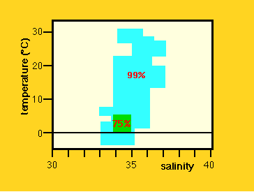 Figura 5.1
The discussion of the previous lectures concentrated on air/sea interaction processes and therefore addressed the distribution of temperature and salinity only in the surface layer, where regional and seasonal variations are large. However, most of the ocean is filled with water of relatively uniform temperature and salinity (Figure 5.1).
If the surface temperature is very low, convection from cooling can reach deeper than the surface layer. This situation is encountered in the polar regions where cold water sinks to the bottom of the ocean. This process replenishes the deeper waters and is responsible for the currents below the upper kilometre of the ocean. Areas of deep winter convection are the Weddell Sea and the Ross Sea in the Southern Ocean and the Greenland Sea and the Labrador Sea in the Arctic region.
The average ocean temperature is 3.8º C; even at the equator the average temperature is as low as 4.9º C. The layer where the temperature changes rapidly with depth, which is found in the temperature range 8 - 15º C, is called the permanent thermocline. It is located at 150 - 400 m depth in the tropics and at 400 - 1000 m depth in the subtropics. (Figure 5.2) shows the temperature and salinity distribution in a meridional section through the Pacific Ocean as an example. Notice the uniformity of both properties below 1000 m depth. Notice also that in many ocean regions, temperature and salinity both decrease with depth. A decrease in temperature results in an increase of density, so the temperature stratification produces a stable density stratification. A decrease in salinity, on the other hand, produces a density decrease. Taken on its own, the salinity stratification would therefore produce an unstable density stratification. In the ocean the effect of the temperature decrease is stronger than the effect of the salinity decrease, so the ocean is stably stratified.
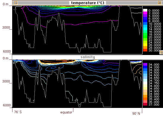 Figure 5.2
In contrast to the subsurface temperature distribution, the subsurface salinity distribution shows intermediate minima. They are linked with water mass formation at the Polar Fronts where precipitation is high; details will be discussed later in the course. At very great depth, salinity increases again because the water near the ocean bottom originates from polar regions where it sinks during the winter; freezing during the process increases its salinity.
Light and sound are two principal carriers of information used in human and animal communication. On land, sound is attenuated over much shorter distances than light, which is therefore the preferred choice for long-distance communication. The reverse situation is found in the ocean: While light does not penetrate very far in water, sound can travel over large distances and is therefore used for various purposes, such as depth sounding, communication, range finding and underwater measurement, by animals and humans alike. Detailed information on the speed of sound (ie the phase velocity of the sound waves) is essential for such applications.
The sound speed c is a function of temperature T,salinity S and pressure p and varies between 1400 m s-1 and 1600 m s-1. In the open ocean it is influenced by the distribution of T and p but not much by S. It decreases with decreasing T, p and S. The combination of the variation of these three parameters with depth produces a vertical sound speed profile with a marked sound speed minimum at intermediate depth: Temperature decreases rapidly in the upper kilometre of the ocean and dominates the sound speed profile, i.e. c decreases with depth. In the deeper regions (below the top kilometre or so) the temperature change with depth is small and c is determined by the pressure increase with depth, ie c increases with depth. Vertical changes of salinity are too small to have an impact; but the average salinity determines whether c is low (if the average salinity is low) or high (if the average salinity is high) on average.
Figure 5.3 shows examples of sound speed profiles. Note the curves for the Weddell Sea and the Mediterranean Sea: The Weddell Sea does not have a thermal stratification, hence no temperature effect on c. The Mediterranean Sea demonstrates the effect of salinity on c: The profile is similar to those of other tropical ocean regions, but the higher salinity of the Mediterranean Sea increases c at all levels.
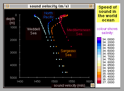 Figure 5.3
If your browser supports JavaScript you can check the dependence of the speed of sound on temperature, salinity and pressure with this sound speed calculator: Enter a value for temperature, a value for salinity and a value for pressure and press the calculate button. By comparing your result with the sound speed profiles of different ocean regions (Figure 5.3) and experimenting you can get a feeling for the temperatures and salinities which must exist in these regions in order to produce the observed sound speeds.
| Sound Speed Calculator | ||
| Enter your values: | ||
| temperature (º C): | ||
| salinity: | c = m s-1 | |
| pressure (dbar): | ||
Calculation based on Fofonoff, P. and R. C. Millard Jr (1983) Algorithms for computation of fundamental properties of seawater.Unesco Tech. Pap. in Mar. Sci. 44, 53 pp.
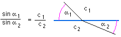
Sound propagates along rays (just as light does). Thus, the laws of geometrical optics are applicable to sound:
As the stratification in the ocean is nearly horizontal, sound propagation in the vertical is practically along a straight path. This is the basis for echo sounding: The depth is known if the mean sound velocity is known. A first estimate is 1500 m s-1; available tables list corrections for the various areas of the world ocean.
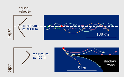 Figure 5.4
Figure 5.4 gives examples of horizontal sound paths. The first diagram shows sound propagation at the depth of the sound speed minimum (usually about 1000 m). Sound rays bend back towards the depth of minimum sound speed and travel at that depth over large distances (they can traverse entire oceans). This sound channel is known as the SOFAR (SOund Fixing And Ranging) channel. Before the introduction of the Global Positioning System (GPS) the SOFAR channel was used to locate ships and aircraft in distress, and for tracking floats (with two or more receivers) for the study of ocean currents. The second diagram shows a situation where a mixed layer of uniform temperature (typically about 100 m thick) is found on top of the normal temperature stratification. In this case sound speed increases below the surface due to the increase in pressure before the normal decrease due to temperature takes over. The resulting sound speed maximum at about 100 m depth creates a shadow zone, since all sound rays bend away from that depth.
Justus von Liebig discovered what has become known as the "Minimum Law" of agriculture, that ecosystem productivity is limited by the nutrient which is exhausted first. On land the limiting element is either phosphorus, nitrogen or potassium (depending on soil type). In the ocean Liebig's Law indicates that the limiting elements should be
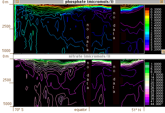 Figure 5.5
phosphorus (as organic or anorganic phosphate)
nitrogen (as nitrate, nitrite, and ammonia)
silicon (as silicate)
On land nutrients enter the soil by decomposition of dead organic matter. In the ocean nutrient uptake by plants (phytoplankton) occurs in the euphotic zone (the surface layer reached by sunlight) where photosynthesis takes place. Most nutrients are removed from the euphotic zone and transferred to the deeper ocean as dead organisms (detritus) sink to the ocean floor. In the deeper layers organic matter is remineralized, ie nutrients are brought back into solution. This process requires oxygen. Thus,
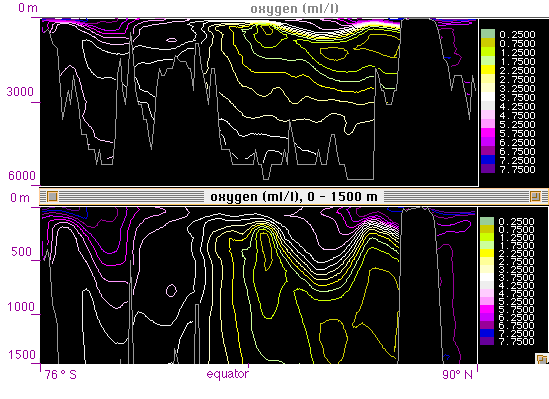 Figure 5.6
Oxygen and nutrients are linked in a cycle of uptake and release, so a fixed ration of their concentrations is found in open ocean water:
| AOU : C : N : P = | 212 | : | 106 | : | 16 | : | 1 | on atomic weight |
| = | 109 | : | 41 | : | 7.2 | : | 1 | in grams |
AOU (apparent oxygen utilisation) = saturation concentration - observed concentration
C = carbon N = nitrogen P = phosphorus
The last three decades of the last century have seen great progress in the understanding of ocean chemistry, and it has now become clear that phosphate, nitrate and silicate are not the only growth-limiting nutrients in the ocean. In more than 40% of ocean regions biological growth is limited by the supply of iron (Fe). The reason for this difference between land based ecosystems and marine ecosystems is found in the early evolution of the earth.
As described in the Introduction lecture, the composition of the atmosphere is the result of the presence of life on Earth (compare the figure). The first life forms to develop (the prokaryotes, which are basically just molecules surrounded by a membrane and cell wall) found an atmosphere that consisted mainly of carbon dioxide (CO2). They used the chemical elements available in the ocean for storage, transport and transfer of energy. Iron is one of the most abundant elements and became essential to many cellular functions.
The advent of photosynthesis in plants changed the relative distribution of C, O and Fe dramatically. As the oxygen level of the atmosphere increased, the oxygen was initially reduced by the available iron, creating vast deposits of iron oxide in the earth's crust. Eventually the supply of free iron was depleted, and the build-up of oxygen that allowed the evolution of higher life forms began. But primitive marine life still requires Fe for its cell functions, and this explains why in the ocean iron is an additional limiting element and in many situations the limiting factor. Field experiments have shown that oceanic productivity increases dramatically when iron is added to the euphotic zone.