
![]()
![]()
![]()
Short waves (deep water waves) show normal dispersion, i.e. wave speed depends on the period, with the longer period waves moving faster than the shorter period waves (and the longer period waves have the longer wave lengths).
In contrast, long waves (shallow water waves) are non-dispersive: Their wave speed is independent of their period. It depends only on the water depth, in the form
\[ c = \sqrt{ g h} \]
($c$ is wave speed, $h$ water depth, $g$ gravity).
The velocity structure in a long wave is described by
\[ U = \dfrac{g\; \zeta}{\sqrt{g h}} \]
where $\zeta$ is the time dependent surface elevation (wave amplitude) and $U$ the horizontal particle velocity. It follows that $U$ is independent of depth and the vertical particle velocity varies linearly with depth. Particles move on very flat elliptic paths in nearly horizontal motion.
Tsunamis are long waves generated by submarine earthquakes. Tsunami is Japanese for "harbour wave". They are often called tidal waves; but this is a misnomer, since tsunamis have nothing to do with tides.
Before 2004 the strongest tsunami in known history was produced by the eruption of the Krakatau of the Sunda Island group in 1883. It reached a wave height of 35 m and claimed 36,830 lives. Four tsunamis with heights in excess of 30 m have been documented in the Pacific Ocean since 684 A.D. A strong tsunami in the Atlantic Ocean was observed in 1755 after an earthquake near Lisbon (Portugal).
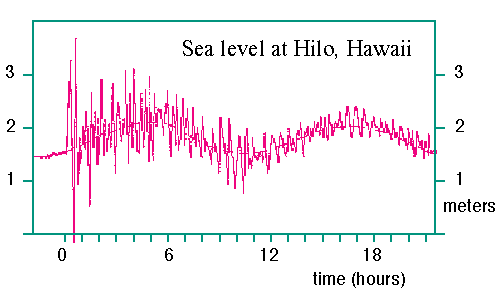
In the vicinity of the epicentre of an earthquake, tsunamis can result in extreme wave heights. Once they reach the open ocean and travel through deep water tsunamis have extremely small amplitudes but travel fast, in 4000 m water depth at about 700 km/h. (This speed can be estimated by using the wave speed equation given above: We have g = 9.8 m s-1, h = 4000 m, so (9.8 x 4000)1/2= 200 ms-1= 700 km/h.) On approaching a coast they build up wave height again through shoaling. The period of tsunamis is in the range 10-60 minutes. Figure 10.1a shows a record of a tsunami from an Alaskan earthquake recorded in Hawaii.
Tsunamis were used to estimate the depth of the ocean in 1856, when direct depth measurements were virtually impossible, by observing their phase speed. The result for the North Pacific was 4200 - 4500 m, which was a considerable improvement on the previous estimate of 18,000 m.
 Figures 10.1 a-c
The most destructive tsunami known occurred on 26 December 2004. It was generated by an earthquake in the vicinity of the Andaman Islands and northern Sumatra and caused death and destruction in countries around the Indian Ocean. The death toll is estimated at between 265,000 and 320,000, although a final accurate figure may never be known.
Because of the destructive force of tsunamis, a tsunami warning system has been set up. It uses seismographic observations of earthquakes and calculates arrival times around the coastlines of the oceanic basin. Another possibility is the monitoring of compression waves linked with volcanic eruptions; they travel at the speed of sound (1500 m s-1) in the SOFAR channel. No warning system is available for areas in the vicinity of the epicentre.
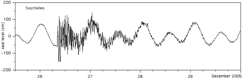
Figure 10.1b shows the passage of the tsunami of 26 December 2004 through the Seychelles. You can also view some photos showing the impact of major historical tsunamis and animations of tsunami propagation derived from a numerical model.
Seiches are standing waves in closed or semi-enclosed basins. Consider a basin of length L and depth h with long wave speed
\[ c = \sqrt{ g h} \]
The time it takes a wave to travel through distance L is
\[ \dfrac{L}{\sqrt{g h}} \]
Reflection occurs at the wall and the same time is needed to return to the starting point. Thus the basic period of a standing wave in the basin is
\[ T_1 = \dfrac{2 L}{\sqrt{g h}} \]
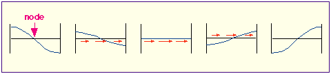 Figura 10.2
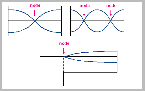 Figura 10.3
This is the period for the free oscillation of lowest (first) order. Higher order waves are possible with periods $T_1/n$ for order n. The order is given by the number of nodes in the surface oscillation. Figure 10.2 shows the first order seiche (of period $T_1$), Figure 10.3 the second order seiche (of period $T_2 = 1/2 T_1$).
Figure 10.4 shows a first order seiche in the Baltic Sea, where such oscillations of water level are usually produced by storms systems travelling across. The storm triggers a free oscillation (seiche) which then continues for several days before it is damped by bottom friction.
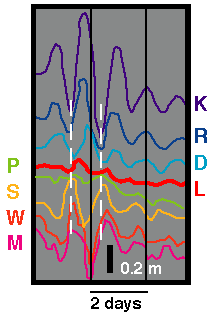 Figura 10.4
If the basin is open, the connecting line to the open sea has to be a node (Figure 10.3). The corresponding period for the lowest order wave is therefore twice that of the lowest order seiche that would exist if the basin were closed (The effective wave length is twice the length of the basin). It is determined in analogy to the frequency determination of organ pipes and is
\[ T_1 = \dfrac{4 L}{\sqrt{g h}} \]
Higher order seiches, with period $T_1/n$, are again possible.
It was said before that waves are periodic movements of interfaces. If the water column consists of an upper layer and a denser lower layer, the interface between the layers can undergo wave motion. This motion, which does not affect the surface and mostly is not observable at the surface, is an example of an internal wave.

 Figures 10.5 - 10.6 - 10.7
The restoring force for waves is proportional to the product of gravity and the density difference between the two layers (the relative buoyancy). At internal interfaces this difference is much smaller than the density difference between air and water (by several orders of magnitude). As a consequence, internal waves can attain much larger amplitudes than surface waves. It also takes longer for the restoring force to return particles to their average position, and internal waves have periods much longer than surface gravity waves (from 10 - 20 minutes to several hours, compared to several seconds or minutes for surface gravity waves). In contrast to surface waves in which horizontal particle velocities are largest at the surface and either decay quickly with depth (in deep water waves) or are independent of depth (in shallow water waves), horizontal water movement in internal waves is largest near the surface and bottom and minimal at mid-depth.
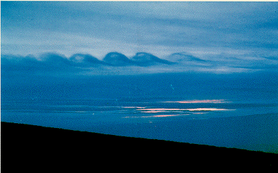
Internal waves can often be observed in the atmosphere, where they travel on the interface between warm and cold air. Figure 10.5 and Figure 10.6 show two examples.
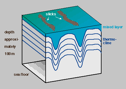
Figure 10.7 shows an example of an internal wave travelling on the seasonal thermocline in coastal waters. Such waves typically have wave lengths of several tens of metres and periods of about 30 minutes.
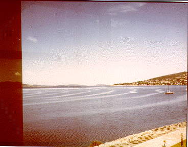 Figura 10.8
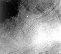 Figura 10.9
The most common internal waves are of tidal period and manifest themselves in a periodic lifting and sinking of the seasonal and permanent thermocline at tidal rythm. In some ocean regions their surface expressions, produced by convergence over the wave troughs, is visible in satellite images (Figure 10.9).