

![]()
![]()
Estuaries are often used as disposal sites for unwanted biological or industrial products, usually referred to as waste. If such waste enters the estuarine ecosystem but is potentially harmful to life or has potentially detrimental effects on its health it is usually called a pollutant.
This chapter discusses basic methods to understand the distribution of pollutants in estuaries. It is important to realise that these methods can be a management tool and an aid in decision making but nothing more; they should not be seen as the starting point for decision making. Whether a material constitutes waste or not depends on many factors. What appears as waste to one individual can constitute a valuable resource to another. The first consideration before a decision is made to introduce a pollutant into an estuary should therefore be what other alternatives exist. The questions that should be asked are: Can the "waste" be put to good use somewhere, so that its introduction into the estuary is not necessary? If not, is it a harmless substance or a pollutant? If it is potentially harmful, is disposal in the marine environment the most appropriate way of dealing with the problem? The methods discussed here can then help to evaluate the cost and environmental impact of all possible ways of dealing with the problem.
The usual way of controlling negative impacts of pollutant dispersal in estuaries is by monitoring its concentration in the water and making sure that the concentration does not exceed a certain level above which the pollutant is considered harmful. This problem consists of two parts, the near field and the far field. The near field problem considers technical details of pollutant outfall design and ways to inject the pollutant into the estuary from a point source in such a way that its concentration is reduced as rapidly as possible. This is an engineering task, and the near field problem is therefore not concidered in oceanography. The far field problem studies the distribution of the pollutant through the entire estuary, starting from the disposal site not as a point source but as an extended source of uniform concentration across the estuary depth and width. The far field problem thus assumes that the engineering design of the pollutant outfall achieves reasonably uniform distribution over a sizeable section of the estuary and uses this situation as the starting point for the analysis.
If the concentration of a pollutant at the location where it is introduced into the estuary is known, its distribution through the estuary can be predicted from theoretical considerations. To understand how this is done it is useful to begin with a look at the distribution of salt and freshwater in the estuary. Let us consider salt as a "pollutant" and follow its path through the estuary. Its source is at the estuary mouth, where its concentration is given by the oceanic salinity $S_0$. The salt enters the estuary with the net water movement of the lower layer. As it moves up the estuary its concentration decreases through turbulent diffusion; in other words, the salt "pollutant" is diluted with freshwater that comes down from the river. We can normalise the salt "pollutant" distribution along the estuary by making it independent of its original "concentration" $S_0$ and define the salt water fraction $s$ as $s = S/S_0$, where S is the local depth averaged salinity at any arbitrary location in the estuary. This normalised salt concentration or salt water fraction decreases from 1 at the mouth to 0 at the inner end of the estuary.
In a similar fashion we can consider the freshwater introduced by the river as a "pollutant" and follow its path through the estuary. Its source is at the inner end of the estuary, where its normalised concentration or fresh water fraction $f$ is equal to 1. The freshwater then moves down through the estuary with the net water movement in the upper layer, reaching a concentration of zero at the estuary mouth. Since the estuary only contains salt water and freshwater, the salt water fraction and the fresh water fraction always add up to 1 locally, which means that we have $f + s = 1$. (Note that this is in accordance with the definition of the freshwater fraction given in the discussion of the flushing time in Chapter 15.)
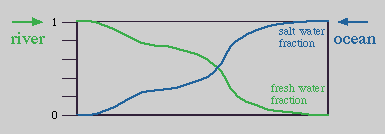 Figure 16.5
Figure 16.1 gives a graphical representation of the distribution of the two "pollutants" salt water and fresh water. One "pollutant" has its source at the estuary mouth and diffuses upstream; the other "pollutant" has its source at the estuary's inner end and diffuses downstream.
Not all pollutants are introduced into the estuary through the river or from the ocean. Before discussing the situation where a pollutant is released into the estuary at some arbitrary point along its shoreline we note that we can distinguish three classes of marine pollutants. Conservative pollutants are substances that are inert in the marine environment; their concentrations change only as a result of turbulent diffusion. (Salt and freshwater can be considered such substances.) Non-conservative pollutants undergo a natural decay; their concentration depends not only on turbulent diffusion but also on the time elapsed since their introduction into the environment. The concentration of coupled non-conservative pollutants depends on turbulent diffusion and natural decay, which both act to decrease their concentration, and on the availability of other substances in the environment, which allow the concentration to increase over time.
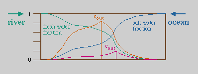 Figure 16.2
A conservative pollutant released at a point between the inner end and the mouth of the estuary will spread through turbulent diffusion in both directions, downstream and upstream. Its diffusive behaviour is no different from the diffusive behaviour of salt or fresh water. In the upstream direction it diffuses in the same way as the salt water diffuses upstream, while in the downstream direction it follows the freshwater diffusion. If its concentration at the outlet is $c_{out}$, its concentration C in the estuary upstream from the release point is thus proportional to the salt fraction, while downstream from the release point it is proportional to the freshwater fraction (Figure 16.2):
upstream: $ C = c_{out} (S / S_{out})$
downstream: $ C = c_{out} (F / f_{out} )$
Here, $S_{out}$ is the vertically averaged salinity at the outlet location and $f_{out}$ the fresh water fraction at the outlet location. This shows that it is possible to predict the distribution of a pollutant in the entire estuary if the salinity distribution is known. The equation assumes steady state conditions, ie continuous release of the pollutant at the constant concentration $c_{out}$.
The concentration of non-conservative pollutants decreases even in the absence of diffusion, through either biochemical or geochemical reaction. An example for such a situation would be the concentration of coliform bacteria released through a sewage outlet. The relationship between the concentration $C$ of such a pollutant, the salinity $S$ and the fresh water fraction $f$ is not as straightforward as in the case of conservative pollutants, but concentration levels are always lower than those derived from the conservative case.
An estimate for the concentration can be determined by subdividing the estuary into compartments. If the compartments are chosen such that the ratio $r$ of the fresh water volume $V_f$ in the compartment and the volume of fresh water $R$ introduced by the river into the estuary over one tidal cycle is constant ($r = V_f/R = constant$), it can be shown that the concentration of a non-conservative pollutant can be approximated by an equation for the concentration in each compartment:
upstream: $ \quad C_p = c_{out} \dfrac{S}{S_{out}} \left(\dfrac{r}{1 - (1-r)e^{\;kT}} \right)^{n+1-p} $
downstream: $ \quad C_p = c_{out} \dfrac{f}{f_{out}} \left(\dfrac{r}{1 - (1-r)e^{\;kT}} \right)^{p+1-n} $
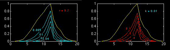 Figure 16.3
In this equation, compartments are numbered from the inner end of the estuary, $n$ is the compartment containing the outfall, and $p$ is the compartment where the concentration is evaluated. $T$ is the tidal period and $k$ the decay constant for the pollutant. The larger $k$, the faster the decrease of the concentration over time. $k = 0$ represents the case where there is no independent decrease without diffusion, or the case of a conservative pollutant. Figure 16.3 compares this behaviour with that of a conservative pollutant. Note that for $k = 0$ the equation for the concentration reduces to
upstream: $ C = c_{out} (S / S_{out})$
downstream: $ C = c_{out} (F / f_{out} )$
which is the same equation that was derived for the conservative pollutant.
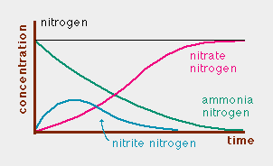 Figure 16.4
Biochemical or geochemical processes do not only reduce the concentration of a non-conservative pollutant, they often also give rise to an increase in the concentration of another substance, which in turn may produce a third substance as a result of its own decay, and so on. Whether this chain of events constitutes pollution or not depends on the degree of harmfulness of each substance. Ammonium nitrogen, for example, is used as a fertiliser on land. Under natural conditions it convertes to nitrate (Figure 16.4), which is also considered a nutrient.
The introduction of nutrients into the marine environment does not automatically constitute pollution. But when nitrate and other nutrients are again mineralised in sea water this process requires oxygen, which is not in unlimited supply in the ocean. Too much nutrient can lead to such a reduction of oxygen levels that the lack of oxygen can become a threat to marine life. Under such circumstances nutrients have to be regarded as pollutants. The chain of events triggered by their presence is then an example of a system of coupled non-conservative pollutants.
The description of the concentration distribution of coupled non-conservative pollutants requires the solution of a coupled system of differential equations, a task well beyond the scope of these notes. An example will have to suffice to demonstrate the principle. Consider a sewage outfall that introduces household effluent into an estuary. The effluent concentration decreases with time, due to oxydation of the organic material. We can express the amount of effluent introduced in units of equivalent Biochemical Oxygen Demand (BOD) as the primary pollutant.
While the Biochemical Oxygen Demand decreases as the effluent concentration is decreased, the result is a reduction of the oxygen concentration in the estuary. An appropriate measure of the stress exerted on the oxygen supply is the Dissolved Oxygen deficit (DO deficit), which expresses how much the oxygen concentration falls below the oxygen saturation level (the highest possible level of oxygen content at the prevailing temperature and salinity). Because lack of oxygen poses a threat to marine life, the DO deficit is then the second in the chain of coupled pollutants.
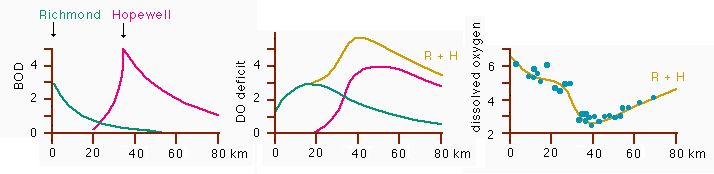 Figure 16.5
Figure 16.5 shows an example from a situation in an estuary during the 1960s. The DO deficit produced by two sewage outfalls was so high that in parts of the estuary dissolved oxygen levels fell below levels considered safe for marine life. An estuary that is treated in such a way cannot sustain a large variety of healthy fish and other marine life forms. Many estuaries are still recovering today from inconsiderate treatment experienced several decades ago, particularly if the waste outfalls contained more inert materials such as heavy metals or pesticides which accumulate in the sediment and can only be removed through mechanical means such as dredging.