
![]()
![]()
In comparison to the open ocean, the shelf and the coastal zone are an extraordinarily energetic environment. Variations of water temperature, salinity, sea levels and currents are all more pronounced here than at large distance from the coast. This is partly the result of an enhanced response of the coastal zone to the forcing experienced by all oceanic regions. Tides, for example, exist everywhere in the ocean, but tidal currents are strongest in the vicinity of the coast.
There is another class of variations in the current field of the coastal ocean. These variations are not an enhancement of forcing mechanisms that operate everywhere in the world ocean; they are the result of features of the coastal ocean itself. Understanding the dynamics of these processes requires advanced analysis of ocean physics and pushes the limits of the introductory level of these lecture notes. This chapter attempts to give a summary of an important class of current variations known as coastal trapped waves. These waves are responsible for most of the observed variability of the currents on the shelf in some regions, and it is essential to include them in a discussion of the coastal ocean.
The starting point for an understanding of the generation and propagation of coastal trapped waves is the open ocean where the basic balance of forces is that of geostrophy. This balance establishes a situation where the pressure gradient force acts in a direction perpendicular to the direction of flow and is balanced by the Coriolis force, which also acts in a direction perpendicular to the flow and in the opposite direction to the pressure gradient force. As discussed in chapter 2, this leads to a situation where a current in the northern hemisphere has the high pressure on its right, and a current in the southern hemisphere has the high pressure on its left.
 Figure 8.1
One consequence of geostrophy is that in the open ocean, isolated centres of high or low pressure form closed circulation cells known as eddies. Figure 8.1 shows the circulation around eddies in the northern and southern hemisphere. Frictional forces are generally small in the open ocean, and the current can circulate around the pressure centres for more than a year with very little loss of energy. Eddies in the open ocean are therefore long-lived features. They can stay in the same place for long periods of time and change their location only when they are moved around by the ocean current. (note)
In the coastal ocean high and low pressure centres do not have to be surrounded by uniform pressure on all sides (as is the case with eddies in the open ocean) but can "lean against the coast". This means that the current can flow along the isobars only on one side of the pressure centres and has nowhere to go when it runs into the coastline. The result is transport of water from one side of the pressure centre to the other, or a lowering of the sea level on one side and a rise of sea level on the other. A change in sea level is equivalent to a change in pressure, so the pressure centres are no longer stationary but have to move along the coast. Figure 8.2a demonstrates that this results in movement towards the equator on the western side and in poleward movement on the eastern side of the oceans. Note that the direction of movement is the same for high pressure centres and for low pressure centres.
 Figure 8.2
The movement of high and low pressure centres along the coast is known as a Kelvin wave. Kelvin waves have their largest amplitude at the coast. On the western coast of an ocean they can only propagate towards the equator, while on the eastern coast they propagate only away from it. Their amplitude falls off rapidly (exponentially) towards the open ocean, so their presence is only felt within a narrow strip of less than 100 km width along the coast. Their period is in the range of several days to a few weeks, which means that they manifest themselves through slow changes of water level and a reversal of the inshore current at a rate of once a week or so, as successive regions of high and low pressure pass the observation point.
A special situation occurs at the equator. Here the regions of high and low pressure cannot lean against a coast, but the current cannot circulate around them because the Coriolis force acts in opposite directions in the two hemispheres and the geostrophic balance is therefore reversed. As a result the current flows eastward on either side of a high pressure cell and westward on either side of a low pressure cell. (Figure 8.2a) This leads again to net transport of water and a shift of the pressure centres, which is now eastward for both high and low pressure centres. These waves are known as equatorial Kelvin waves. They have similar periodicity as coastal Kelvin waves but propagate at much larger speed. An equatorial Kelvin wave traverses the entire Pacific Ocean in less than two months.
 Figure 8.3
Figure 8.3 shows observations of Kelvin waves travelling along the eastern coast of the Atlantic Ocean. The waves are believed to be generated in the equatorial region off the coast of Brazil and travel along the equator to reach Africa in a matter of weeks. When they arrive at the African coast they continue poleward along the coast, eventually reaching the coast of Ghana where the coastline has a zonal orientation, so the waves propagate eastward there.
 Figure 8.4
Coastal Kelvin waves depend on the existence of a coast against which they can "lean" but do not require the existence of a shelf region. They can exist equally well in regions where the continent falls off to great depth into deep trenches, as is the case, for example, along the coast of Chile and Peru (Figure 8.4). The presence of a shelf gives rise to another class of waves known as coastal trapped waves. The existence of these waves depends entirely on the presence of a region of shallow ocean between the coast and the deep ocean. To be more specific, these waves exist because the shelf is not of uniform depth but falls off gradually towards the deep ocean; in other words, a major ingredient of their dynamics is the presence of a sloping sea floor or a bottom gradient.
To understand how these waves are generated we begin by looking at the general situation on the shelf. On a rotating earth the wind produces water movement in the Ekman layer. The current direction in the Ekman layer varies with depth, but the net effect of water movement in the layer is perpendicular to the wind. If a shelf region is exposed to variable wind, such that the wind component parallel to the coast varies periodically in time, this will produce periodic upwelling and downwelling at the coast. Below the Ekman layer this results in periodic onshore and offshore movement of the entire water column (Figure 8.5).
figura 8.5).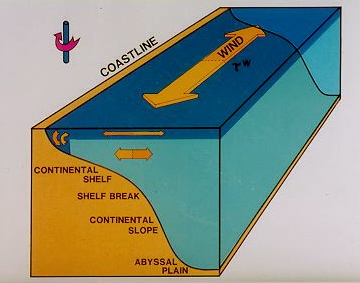 Figure 8.5
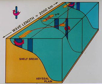 Figure 8.6
If the depth of the shelf is constant, the water below the mixed layer will simply move in and out in passive response to the wind forcing and associated periodic upwelling and downwelling. On a shelf with a sloping bottom the water column will grow in length and get slimmer as it moves offshore and shrink and widen as it moves inshore. Because the water column finds itself on the rotating earth it carries a certain amount of angular momentum. Conservation of angular momentum is one of the basic laws of physics, so the water column cannot change its angular momentum at will. Just as an ice skater performing a pirouette maintains angular momentum by rotating faster when drawing the arms in and slower when stretching them out, the water column will start to rotate when it gets slimmer and slow down when it widens. The degree of rotation around a vertical axis is measured by a quantity known as vorticity. Offshore and inshore movement of a water column on a sloping shelf below the Ekman layer is thus associated with a continuous change of vorticity. Figure 8.6 shows this for a situation where the wind direction alternates between equatorward and poleward along the coast over a distance of about 2000 km, the typical size of atmospheric weather systems that affect the coastal zone. It shows that an imaginary line parallel to the coast somewhere at a mid-shelf location is deformed into a wavy line in response to the wind forcing.
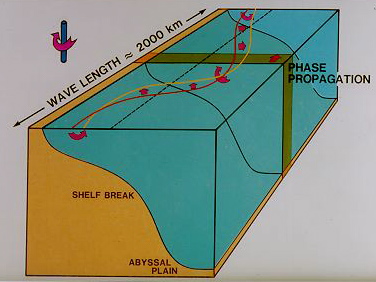 Figure 8.7
On a shelf with constant depth the imaginary line would oscillate in response to periodic wind forcing between two wavy lines like the string of a guitar or violin. In other words, it would undergo a standing oscillation. Figure 8.7 demonstrates how the tendency for water movement on a sloping shelf to induce changes in vorticity translates into water movement along the coast. The result is a propagating oscillation: The wavy line does not return to its original position but shifts along the coast.
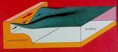 Figure 8.8
Note that we assumed that the wind forcing is periodic but stationary with respect to the shelf: The wind changes from poleward to equatorward and back as a function of time, but the wind field does not move along the coast. The presence of a sloping shelf results in the generation of propagating waves which will leave the region of periodic wind forcing and will be observed as periodic water movement further along the coast where the variations in the wind field are no longer related to them. This water movement is the coastal trapped wave. Figure 8.8 shows its shape.
 Figur3s 8.9-11
Like Kelvin waves, coastal trapped waves can only propagate towards the equator on the west coast of the oceans and towards the poles on the east coast of the oceans. (They can obviously not exist at the equator.) They have similar periods as coastal Kelvin waves (several days to 2-3 weeks) and similar wave lengths (of the order of 2000 km, determined by the atmospheric weather patterns) but a different wave profile (with a relative maximum of sea level oscillation over the shelf edge). If the stratification of the shelf waters is taken into account, their shape and associated currents are modified further, and they can have strongest currents at mid-depth. Because the stratification in shallow water is strongly affected by the seasons, the effect of coastal trapped waves on shelf currents and sea level variations can vary with the seasons.
Coastal trapped waves can make a significant contribution to the observed variability of sea level and currents on the shelf. Figure 8.9 demonstrates this with observations from the southern part of the east coast of Australia where a dedicated experiment for the study of these waves took place in the 1980s. When the experiment was designed it was assumed that the waves were locally forced by fluctuations of the wind. Since then it has become evident that the waves continue as free waves towards the equator and are observed along the northern part of the coast (Figure 8.10), where they are not related to local wind variations. Sea level variations along the Indian Ocean coast of Australia can be followed along half the continent as coastal trapped waves (Figure 8.11). There is no doubt that coastal trapped waves are a major feature of most shallow shelves.