
![]()
![]()
Up to this point, our discussion of the dynamics of the coastal ocean included the effects of shallow water and the presence of a coastline. The last chapter introduced the additional aspect of coastline shape, addressing in particular the effect of headlands and promontories. We now turn to another topographic feature that can influence the circulation.
In a discussion of deep ocean dynamics, the effect of islands on the oceanic flow field is rarely considered. Most islands are part of the continents and therefore located on the continental shelf. The number of true deep ocean islands is very small, and when compared to the size of the ocean basins, they are minuscule and of no consequence for the oceanic circulation. On the shelf, the impact of islands on currents and stratification can be considerable, and a discussion of the dynamics of the coastal ocean would be incomplete without some discussion of island effects. As in previous chapters, the best way to understand the effects of islands in shallow water is by starting from the situation in the deep ocean.
 Figure 7.1
To begin with, consider a current of constant speed and direction flowing past an idealized island with vertical coasts. Islands are obstacles to the flow; they force water particles to depart from the straight path which they would follow in the absence of the island. By deviating from its intended path the particles experience an acceleration perpendicular to their original direction. At the same time, the particles experience friction as they try to pass around the island. The path of an individual particle around an island will thus be determined by the balance of two forces, the force associated with the acceleration that causes its departure from a straight path, known as the inertial force, and the frictional force associated with the frictional boundary layer around the island (Figure 7.1).
The frictional boundary layer is produced by the same process that establishes frictional boundary layers at the ocean floor (water flowing past a stationary object experiences a drag force; see Chapter 3). However, unlike the ocean floor which spreads horizontally, the stationary surface presented by the idealized island has a vertical orientation. As a consequence, while currents in the boundary layer above the ocean floor show a vertical gradient (they increase from zero at the bottom to their open ocean value at some vertical distance from the ocean floor), currents in the frictional boundary layer attached to the island show a horizontal gradient (they increase from zero at the vertical coast to their open ocean value at some horizontal distance from the island). We can use eqn. (3.2) to determine the thickness of the boundary layer if we replace the coefficient A that describes the vertical exchange of momentum by its horizontal equivalent $A_h$, the coefficient of horizontal momentum exchange. $A_h$ represents the effect of turbulent mixing in the horizontal plane. Compared to the small overturning eddies that form the basis for vertical mixing, the eddies responsible for the horizontal mixing of momentum are larger by several orders of magnitude. A typical value for $A_h$ is of the order $10^5\; m^2\; s^{-1}$, giving an associated boundary layer thickness
\begin{equation} d_h = \sqrt{ \dfrac{2 A_h}{f} } \label{eq:dh} \end{equation}
in the range 15 - 150 km. (This leads to the convenient rule of thumb that, expressed in kilometres, $d_h$ is numerically about the same as the thickness $d_E$ derived for surface and bottom boundary layers, expressed in metres.)
 Figures 7.2a-d
The effect of an island on the flow field depends on the relative importance of the inertial and frictional forces. If the frictional force dominates, the particles will be dragged along the island's coast. If the inertial force dominates (ie the acceleration perpendicular to the particles' intended path is large) the particles will be thrown off their paths and the flow will separate from the island. The ratio of inertial force vs. frictional force is known as the Reynolds number Re, a dimensionless number given by
\begin{equation} Re = \dfrac{u\; L}{A_h} \label{eq:reynolds} \end{equation}
where u is the original particle velocity before approaching the island, L the width of the island and $A_h$ the horizontal Austausch coefficient.
The effect of an obstacle on uniform flow under different Reynolds numbers can easily be investigated in a towing tank. It is found that four different types of flow are observed, depending on the value of Re in the experiment. At very small Reynolds number the flow around the obstacle is controlled by friction; it occurs entirely within the frictional boundary layer and is laminar and symmetric (Figure 7.2a). At slightly larger Reynolds numbers the boundary layer separates behind the obstacle, creating a vortex pair with opposite rotation and central return flow (Figure 7.2b). Moderately high Reynolds numbers lead to the formation of a wake, which exhibits wave disturbances or instabilities at its interface with the undisturbed current (Figure 7.2c). Very high Reynolds numbers produce the separation of the vortices from the obstacle; vortices separate in turn from either side and drift away with 80% of the background velocity u, forming a downstream sequence of vortices with alternate sense of rotation known as a von Karman vortex street (Figure 7.2d).
Table 7.1 lists typical values found for a flat plate oriented perpendicular to the flow. Other obstacle shapes produce the same transition from laminar boundary layer flow to vortex pair, wake with wave disturbances and von Karman vortex street; but the change from one type of flow to another occurs at somewhat different Re values. Table 7.1 gives a range of Reynolds numbers observed for a large variety of obstacle shapes.
| flat plate | other shapes | type of flow |
| $Re < 1$ | $Re > 0.5$ | laminar flow, no separation |
| $Re \ge 1$ | $Re > 2 - 30$ | vortex pair with central return flow |
| $Re \ge 10$ | $Re > 40 - 70$ | wake formation with wave disturbances |
| $Re >> 10$ | $Re > 60 - 90$ | von Karman vortex street |
Eddies dissipate energy, and wakes behind obstacles are regions of intense energy dissipation. The energy is withdrawn from the mean flow and has to be replaced if the situation is to remain in a steady state. The laboratory experiments from which the values in Table 7.1 were derived were all done by towing an obstacle through a tank with fluid at rest, so the energy dissipated in the wake is provided by the action of towing the obstacle through quiescent water. In the ocean it can be supplied by the wind field, an internal pressure gradient or the tides.
Towing an obstacle through a tank with fluid at rest does, of course, give the same result as if a uniform current passes a stationary object. However, an important aspect of the flow field in a tank is that the current is uniform in the horizontal and in the vertical. This condition is not met in the ocean. Wind-driven currents exhibit strong vertical current shear. In the deep ocean the total vertical variation of current speed and direction is distributed over a much larger distance than in the coastal ocean. Before attempting to extend the findings from laboratory experiments to the shallow ocean it seems therefore appropriate to look for observations of island wakes and vortex streets in the deep ocean first.
 Figure 7.3
Unfortunately, there are only very few true deep ocean islands, most of them in rather remote locations. Observations of island wakes in the ocean are therefore quite rare. The situation is better in the atmosphere, where island wakes sometimes manifest themselves through cloud patterns that are easily observed from satellites or aircraft. Figure 7.3 shows examples of atmospheric vortex streets behind Guadelupe, an island some 200 km west of Baja California, Mexico.
 Figure 7.4
An observation from an oceanic situation was reported from Johnston Atoll, a deep ocean island located at 16º45'N, 169º31'W, some 100 km southwest of the islands of Hawaii in the North Equatorial Current of the Pacific Ocean. The island is roughly elliptical in shape with an equivalent diametre of 26 km. A vortex street was observed in February 1968 when the North Equatorial Current flowed with 0.6 m s-1. No wake was found eight months later when the current was reduced to 0.15 - 0.20 m s-1 (Barkley, 1972). Location and movement of the vortices were reconstructed from the drift of longlines observed during a six day fishing period. Figure 7.4 shows the reconstruction, indicating a series of vortices with a wavelength (distance between vortices with the same sense of rotation) of 160 km.
Table 7.2 compares Johnston Atoll's wake with an atmospheric wake system observed behind Madeira, the largest island in a group of islands near 32º44'N, 17ºW in the eastern north Atlantic Ocean some 800 km off the coast of Morocco. It is seen that the two islands, which are of comparable size, produce quite similar wakes, because the flow field of the North Equatorial Current in the Pacific Ocean and that of the Trade Winds over the North Atlantic Ocean produce similar Reynolds numbers; the much higher wind velocity is compensated by the much higher atmospheric eddy viscosity. This similarity suggests that the lengths of both wakes are also similar and that Johnston Atoll produces a wake of 600 km total length.
Assuming that the source of energy to sustain the North Equatorial Current comes from the wind field, it was estimated that about 10% of the wind energy supplied to the Pacific Ocean would be dissipated in island wakes if all Pacific islands had von Karman vortex streets at all times. The observations from Johnston Atoll show that this was not the case during October 1968, so the energy dissipation estimate is certainly too high. This confirms our earlier statement that deep ocean islands do not play an important role in the dynamics of the deep ocean.
| parameter | ocean (Johnston Atoll) |
atmosphere (Madeira) |
| effective island diameter | 26 km | 40 km |
| wavelength or pitch of vortex street | 160 km | 190 km |
| width between vortex rows | 55 km | 83 km |
| speed of incident flow | 0.6 m s-1 | 10 m s-1 |
| translation speed of wake | 0.45 m s-1 | 7.5 m s-1 |
| period of eddy pair formation | 4 days | 7.2 hours |
| Reynolds number | 70 | 90 |
| eddy viscosity coefficient | 220 m2 s-1 | 4,400 m2 s-1 |
The principles discussed so far are equally valid for island wakes in shallow water. Wake formation and behaviour are again controlled by the ratio of inertial to frictional forces. The differences become apparent when the details of the frictional processes are addressed. The discussion of the deep ocean situation was based on the assumption that the friction experienced by the flow field originates from the island's coastal boundary. We know from our discussion of Ekman layer dynamics in Chapter 3 that frictional effects are also important in the surface and bottom boundary layers of the ocean. The assumption that the only frictional effects produced by a deep ocean island originate from its (quasi-vertical) coast implies that frictional effects from the surface and bottom boundary layers are negligible in comparison. Quantitatively this is true if these boundary layers make up a negligible fraction of the total water depth or if, in the notation of Chapter 3, $d_E^2 >> H^2$. This condition is no longer satisfied in the coastal ocean under all circumstances. Our task therefore is to compare the inertial force with the frictional force under conditions where Ekman layer depth $d_E$ and water depth H become comparable in size.
The easiest case to consider is the situation where the surface and bottom boundary layers merge and take up the entire water column. All frictional work is then done by turbulent transport of momentum in the vertical direction, and the contribution from the island's coast (assumed vertical as before, to simplify matters), ie the horizontal turbulent transport of momentum, is negligible.
As expressed by eqn. (7.2) the Reynolds number measures the ratio between inertial forces and forces due friction at the coast. The Reynolds number for the situation of the shallow ocean is derived by comparing the inertial force, which remains unchanged, with the frictional force associated with the surface and bottom boundary layers rather than the coastal boudary layer. It turns out as
\begin{equation} Re^s = \dfrac{u\; H^2}{A_v\; L} \label{eq:re} \end{equation}
Here, u and L are the background velocity and the width of the island as before, H is the water depth, and the vertical Austausch coefficient $A_v$ replaces the horizontal Austausch coefficient $A_v$. The superscript s serves as a reminder that this form of the Reynolds number is valid for shallow water.
Because in this form the Reynolds number comes out different from the form given in eqn. (7.2) it is often not recognized as a Reynolds number but given a separate name and symbol, the name "island parameter" and symbol P being most common. This is unfortunate, since both versions of the Reynolds number compare the same balance of forces, between the inertial and frictional forces, under different oceanic conditions (Tomczak, 1988). Use of a different name and symbol gives the wrong impression that the balance of forces in deep and shallow water is different in principle. The term "island parameter" should therefore not be used.
The conclusion from this discussion is that island wakes in shallow water produce the same sequence of flow situations listed in Table 7.1 as islands in deep water and the transition from one flow type to the next occurs at the same Reynolds number values, provided Res is used for shallow water situations. In practice this means that the highly turbulent regimes of wakes with wave disturbances or vortex streets are rarely produced in the coastal ocean. This becomes obvious when eqns. (7.2) and (7.3) are combined into
\begin{equation} Re^s = \dfrac{H^2}{L^2} \dfrac{A_h}{A_v} Re \label{eq:illa} \end{equation}
The ratio $A_h/A_v$ is large, but it is more than compensated by the much smaller value of the ratio $H^2/L^2$, and as a consequence $Re_s$ is always much smaller than Re under otherwise identical conditions.
 Figure 7.5
Observations of the moderately turbulent regime characterized by vortex pairs with central return flow have been reported from various locations. Figure 7.5 shows surface temperatures and currents behind a small island of the Great Barrier Reef of Australia. The background current flowed southeastward, producing two vortices on either side of the island and a strong return flow behind it. The circulation was clearly visible from the air (Figure 7.6),indicated by different coloration in the main eddy. The vortices were not of the same size because the island's orientation was not exactly perpendicular to the flow.
 Figure 7.6
As discussed in detail in Chapter 5, the strongest currents of the coastal ocean are often tidal. Vortex formation is therefore often periodic and occurs on alternate side of islands depending on the direction of the tidal current. The observations shown in Figures 7.5 and 7.6 were taken during the rising tide when the tidal current flows strongly southeastward in the region; they do not persist over a tidal cycle. The intermittent character of tidal island wakes is another reason why fully developed extensive island wakes are not frequent in the coastal ocean
 Figure 7.7
Coastal promontories present obstacles to currents and thus can produce flow fields similar to those observed behind islands. The observed circulation can be considered the equivalent of half an island wake. Figure 7.7 shows observations from a promontory on Whitsunday Island in the Great Barrier Reef. The tidal current is seen flowing northwestward, separating from the coast behind Poppy Point and producing the equivalent of half a vortex pair with return flow.
 Figure 7.8
Island wakes and associated eddies can trap suspended and floating material and particles. Knowing their locations is therefore important for aspects of waste disposal, the positioning of sewer outlets and other applications. Eddies can accumulate plankton and attract fish. Figure 7.8 documents the accumulation of zooplankton in the eddy observed behind Poppy Point (Figure 7.7). The concentration of zooplankton biomass in the eddy (the lee of Poppy Point) increases fivefold over normal concentration levels (as found in Hunt Channel) during the live span of the eddy (strongest currents).
 Figure 7.9
A particularly clear observation of vortex development behind an island was observed in Lake Eyre, a salt lake of southern Australia. Lake Eyre is usually a dry lake indicated by a vast expanse of encrusted salt. When it occasionally floods it reaches a depth of 1 - 2 m. Strong contrast between silt laden water and water formed over the dissolving salt crust provides for excellent flow visualisation (Figure 7.9).
An elegant way to summarize the discussion of this chapter is the use of a flow classification diagram, based on the use of dimensionless numbers representing ratios of forces. Geophysical fluid dynamics is concerned with the motion of fluids on the rotating earth. Since the earth's rotation never changes, it is convenient to use the associated force as a reference. The ratio of the inertial force to the Coriolis force is known as the Rossby number Ro, the ration of the friction force to the Coriolis force is the Ekman number E. We therefore have
\begin{align} Re & = (\text{(inertial force / friction force}) \nonumber\\ & = (\text{inertial force / Coriolis force)/(Coriolis force / friction force}) \nonumber\\ & = Ro / E \label{eq:taula} \\ \end{align}
Theory gives
\begin{equation} Ro = \dfrac{u}{f L},\quad E_v =\dfrac{A_v}{f H^2}, \quad E_h =\dfrac{A_h}{f L^2} \label{eq:nombres} \end{equation}
 Figure 7.10
where $E_v$ compares vertical friction against the Coriolis force and $E_h$ horizontal friction. In deep water vertical friction is negligible, so E in eqn. (7.5) is given by $E_h$ and Re comes out as in eqn. (7.2). In shallow water horizontal friction is negligible, E is given by $E_v$ giving Res as in eqn. (7.3). In both cases the transition between different types of flow past islands can be illustrated in a diagram with ln(Ro) on one axis and ln(E) on the other (Figure 7.10). The difference between deep and shallow water is then reduced to different scaling along one coordinate axis; in deep water E stands for $E_h$, in shallow water for $E_v$.
 Figure 7.11
A situation somewhat similar to that observed behind islands is the occurrence of eddies at the entry point of a swift flowing stream into the coastal ocean. The eddies are produced in this case by the intrusion of a jet-like current into more or less quiescent water. In its purest form this process gives rise to two eddies, one on either side of the outlet, of opposing rotation, so-called bipoles. Figure 7.11 shows an example from the West Australian coast. Their existence can be modulated by tidal currents, which may suppress or sweep away one or both of the bipole eddies at times.
A condition for the formation of bipoles is the rapid disappearance of the jet after entering the coastal sea, which usually occurs only in shallow water under the influence of bottom friction. Bipoles are therefore a feature of the coastal ocean. Strong jet-like currents flowing into the deep ocean, such as the western boundary currents of the major ocean basins, continue over long distances and develop instabilities of a different kind (meandering motion which eventually leads to the formation of single eddies). Bipoles are sometimes observed in the system of western boundary currents of the North Pacific Ocean where the Tsugaru Warm Current passes through Tsugaru Strait and dissipates its energy where it encounters the Kuroshio and Oyashio confluence at the edge of the shelf. This feature is again associated with the disappearance of the jet over the shelf.
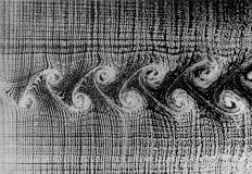 Figure 7.12
We conclude this discussion with an obervation from a laboratory. The behaviour of a fluid which moves past an obstacle has been studied for many decades, and it is surprising that it took until 1990 to notice that fluid behaviour changes quite radically if a second, much smaller obstacle is present in the vicinity of the major one. Figure 7.12 shows that vortex shedding behind a cylinder can be completely suppressed if a second small cylinder is placed in the tank, slightly offset from the main cylinder with respect to theflow direction. The implications for coastal oceanography can only be guessed at this stage. Islands often come in groups in the coastal zone, and the experiment suggests that they can interact quite strongly. Depending on the flow direction relative to the island group, the effect can be to suppress eddies and vortex shedding which would otherwise occur behind a single island. This is another argument why vortex shedding is much less common in the coastal ocean than in deep water.